Part1: Supervised Learning: Basic linear regression

The evolution of Supervised Learning has been very interesting for me. When I was at school, this used to be called curve fitting and the teachers used to give 2D or max 3D problems (for example predict the future house price given the history) so as to visualize on a graph plot. Then during statistics class in college, the same was called Regression and currently everything is some kind of learning and hence I guess the name Supervised Learning. This post is an introduction which uses simple example to understand the basics

As I mentioned, the goal of a Supervised Learning is to predict the future outcomes given the history. A mathematical model, of the form \(y = f(x)\), is used to make an approximation of the real world data. Here \(y\) is called the true label or outcome/output (eg: house prices) and \(x\) is the input or features (eg: number of bedrooms, area of the house in sqaure units etc. that affect the price of the house). Instead of going the traditional way, here I would like to solve the problem of house prediction explicitly and go deeper in to the math. The following is a basic example to understand the concept and in practice several small techniques might need to get a good prediction.

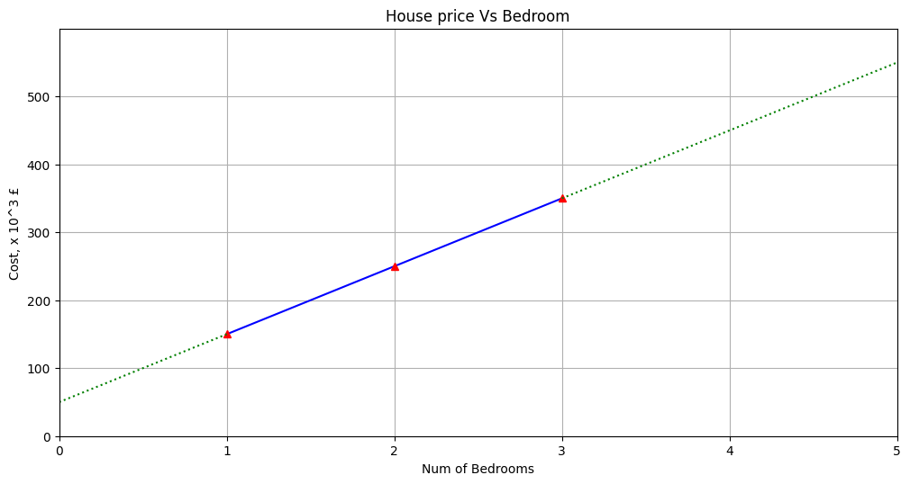
So, imagine if house pricing was as easy as a house costs 50k + 100k per bedroom, so that a 1 bedroom house costs 150k, a 2 bedroom house costs 250k etc. (Here (50, 100) are the weights or parameters that we will find out). We will be given the data, ie.,

house prices, (y): 150k, 250k, 350k
Number of bedrooms, (nB): 1, 2, 3
A plot of the house price vs number of bedrooms is shown here for a better understanding. From this, it is clear that the cost of a 4 bedroom house would be 450k and so on.

Mathematical model 1:

\begin{align} y = w_0 + w_1 \times nB \label{line1} \end{align} where w's are weights that need to be found out and nB’s (or x) are the number of bedrooms. If this can be found out as accurately as possible (by any means), then the Supervised Learning problem can be considered solved. In most general form, eq. \ref{line1} can be represented as

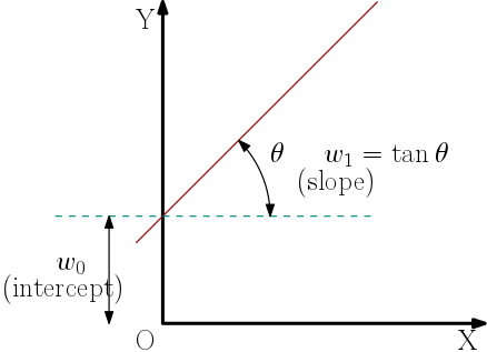
\begin{equation} y = bias~ (intercept) + slope * n_B \nonumber \end{equation}

where w_0 is the bias or intercept and w_1 is called the slope. In matrix form, this can be written as \begin{align} Y &= \begin{bmatrix} 1 & nB \end{bmatrix} \begin{bmatrix} w_0 \nonumber \newline w_1 \end{bmatrix} \newline &= X^Tw \end{align} In this particular case, the matrix equation looks like \begin{align} \begin{bmatrix} 150 \nonumber \newline 250 \nonumber \newline 350 \end{bmatrix} = \begin{bmatrix} 1 & 1 \nonumber \newline 1 & 2 \nonumber \newline 1 & 3 \end{bmatrix} \begin{bmatrix} w_0 \nonumber \newline w_1 \end{bmatrix} \end{align}

Because this is a mathematical model, there would be an error (or residual) and this can be written as \begin{equation} error = w_0 + w_1 \times n_B - y \end{equation} The total error will be the sum of the individual errors which can be written as \begin{align} e &= \sum_{i=1}^{N} (X^Tw - y_i ) \end{align} In the example provided, the error becomes \begin{align} e &= (w_0 + w_1) -150 + (w_0 + 2w_1) - 250 + (w_0 + 3w_1) -350 \nonumber \newline &= (3w_0 + 6w_1) - 750 \nonumber \end{align}

The aim of the regression analysis is to minimize this error and find out suitable value for the parameter w's. The most common technique used to solve this is Optimization where the objective function returns a scalar whose value is greater than or equal to zero. Formulating our problem as an optimization, it can be written as minimizing the sum of squared errors

\begin{align} \rm{Goal:} ~ argmin~ Z = e^Te = \sum_{i=1}^{N} (X^Tw - y_i)^2 \end{align} The sum of the square of the errors is also called Loss function, L

\begin{align} L = e^Te &= (Xw - Y)^T (Xw - Y) \label{eqn:lossfun} \end{align}

Note: The loss function is squared so that the minimum of it is zero. Optimization algorithms (SLSQP, BFGS, fmincon etc.) are designed to search for the parameters (here w’s) that take the value of the function (Z) to a number as close to zero like \(10^{-04}\). (Achieving perfect zero is impossible except for simple problems).

To find the weights, we need to set the gradient of L with respect to w to be zero.

Setting the gradient of eq. \ref{eqn:lossfun} to zero, we get

\begin{align} \frac{\partial L}{\partial w} &= \frac{\partial L}{\partial e} \frac{\partial e}{\partial w} \nonumber \newline &= 2eX\nonumber\newline &= 2(Xw - Y)^TX = 0 \label{eqn:derivative} \end{align} Taking the transpose of eq. \ref{eqn:derivative}, we get

\begin{align} X^T(Xw - Y) = 0 \implies w = (X^TX)^{-1}X^TY \label{eqn:weightvector} \end{align} where the quantity \((X^TX)^{-1}X^T\) is called the left pseudo-inverse

A little bit of code in Python to solve the same

import numpy as np       # library for mathematics (linear algebra)

nB = np.array([1.0, 2.0, 3.0, ])  # Num bedrooms
Y = np.array([150.0, 250.0, 350.0])  # Cost


s = np.ones(len(nB)).reshape(-1,1)
X = np.hstack((s, nB.reshape(-1, 1)))
a = X.transpose() @ X
b = X.transpose() @ Y
w = np.linalg.solve(a, b)  # To find parameters
print(w)

######
[50, 100]

Isn’t this what we started with :-D !!!